Spectral Transformers

One of the biggest challenges for the Transformer architecture, powering modern large language models, is their computational inefficiencies on long sequences. The computational complexity of inference of the attention module scales quadratically with the context length, which can be extremely long in practice, and is thus limiting for the architecture.

The computational bottleneck of transformers gave rise to recent interest in state space models. These alternate architectures are variants of recurrent neural networks that are much faster in terms of inference. Recent works showed their promise in a variety of tasks requiring long context, such as the long range arena benchmark.

In this post we describe a recent methodological advancement for state space models: spectral filtering. We describe the theoretical foundations of this technique, and how it gives rises to provable methods for learning linear dynamical systems with long memory. We then describe how the spectral filtering algorithm can be used for designing neural architectures and preliminary results in long range tasks.

Fundamentals of Sequence Prediction

Stateful time series prediction have been used to model a plethora of phenomena. Consider a sequence of inputs and outputs, or measurements, coming from some real-world machine

\[x_1,x_2, \ldots , x_T , \ldots \ \ \Rightarrow \ \ \ y_1,y_2, y_3 , \ldots, y_T , \ldots\]

For example,

• $y_t$ are measurements of ocean temperature, in a study of global warming. $x_t$ are various environmental knowns, such as time of the year, water acidity, etc.

• Language modeling or translation, $x_t$ are words in Hebrew, and $y_t$ are their English translation

• $x_t$ are physical properties and controls of a robot, i.e. position, velocity, force in various directions, and $y_t$ are the location to which it moves

Such systems are generally called dynamical systems, and the simplest type of dynamics is linear dynamics. A linear dynamical system has a particularly intuitive interpretation as a (configurable) vector field as depicted below (from wikipedia):

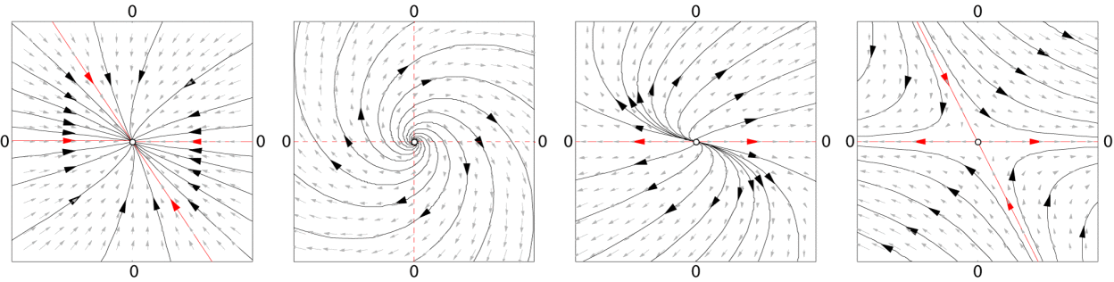
For linear dynamical systems, the output is generated according to the following equations: \(h_{t+1} = A h_t + B x_t + \eta_t\) \(y_{t+1} = C h_t + D x_t + \zeta_t\) Here $h_t$ is a hidden state, which can have very large or even infinite dimensionality, $A,B,C,D$ are linear transformations and $\eta_t,\zeta_t$ are noise vectors.

This setting is general enough to capture a variety of machine learning models previously considered in isolation, such as hidden Markov models, principle and independent component analysis, mixture of Gaussian clusters and many more, see this survey and recent textbook draft.

The Memory of Linear Dynamics

The linear equations governing the dynamics are recursive in nature. An input is multiplied by the system matrix $A$ before affecting the output. The recursive nature of the dynamics means that an input effect $k$ steps into the future will be multiplied by $A^k$, and thus depend exponentially in the eigenvalues of the matrix $A$.

The matrix $A$ is asymmetric in general, and can have complex eigenvalues. If the amplitude of these eigenvalues is $>1$, then the output $y_t$ can grow without bounds. This is called an “explosive” system.

In a well-behaved system, the eigenvalues of $A$ have magnitude $<1$. If the magnitudes are bounded away from one, say at most $1-\delta$ for some $\delta > 0$, then after roughly $\frac{1}{\delta}$ time steps the input decays so much that it won’t have a substantial effect on the output. The quantity $\frac{1}{\delta}$ is referred to as the system memory. This mathematical fact implies that the effective memory of the system is on the order of $\frac{1}{\delta}$. In general, the parameter $\delta$ is unknown a priori and can get arbitrarily small as we approach systems with long range dependencies leading to instability in training linear dynamical systems with a long context. This issue is specifically highlighted in the work of Orvieto et al., who observe that on long range tasks learning an LDS directly does not succeed and requires interventions such as stable exponential parameterizations and specific normalization which have been repeatedly used either implicitly or explicitly in the SSM literature.

Spectral Filtering

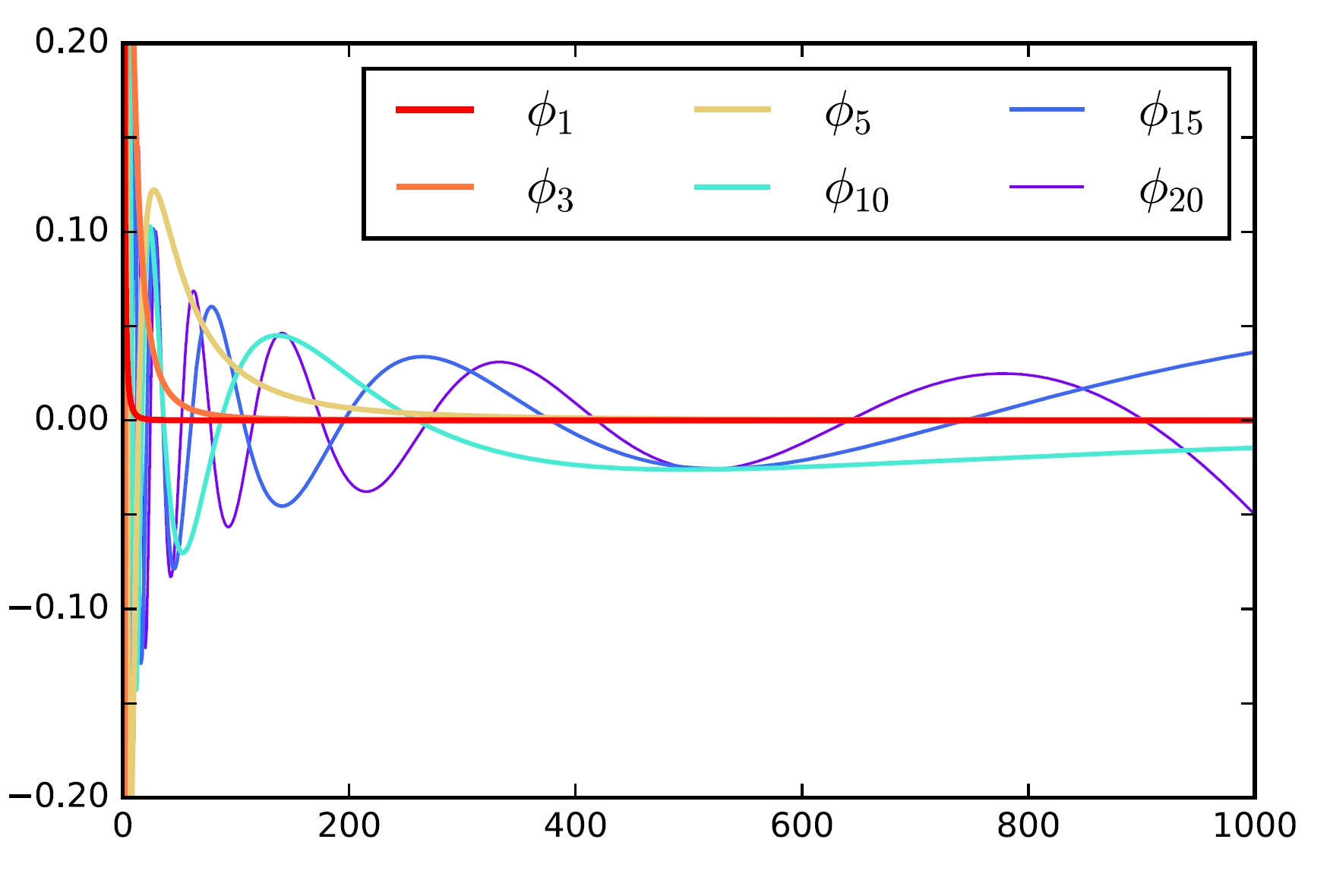
A notable deviation from the standard theory of linear dynamical systems that allows efficient learning in the presence of arbitrarily long memory is the technique of spectral filtering. The idea is to project the sequence of inputs to a small subspace that is constructed using a special structure of discrete linear dynamical systems, where successive powers of the system matrix appear in the impulse response function. We can then represent the output as a linear combination of spectral filters, which are sequence-length sized vectors that given the target sequence length can be computed offline. These spectral-filters are the eigenvectors of a special matrix constructed as the average of outer products of the discrete impulse-response functions. The structure of this matrix implies that it has a very concentrated spectrum, and very few filters suffice to accurately reproduce any signal. This magical mathematical fact is explained in the next section, the filters themselves are depicted here

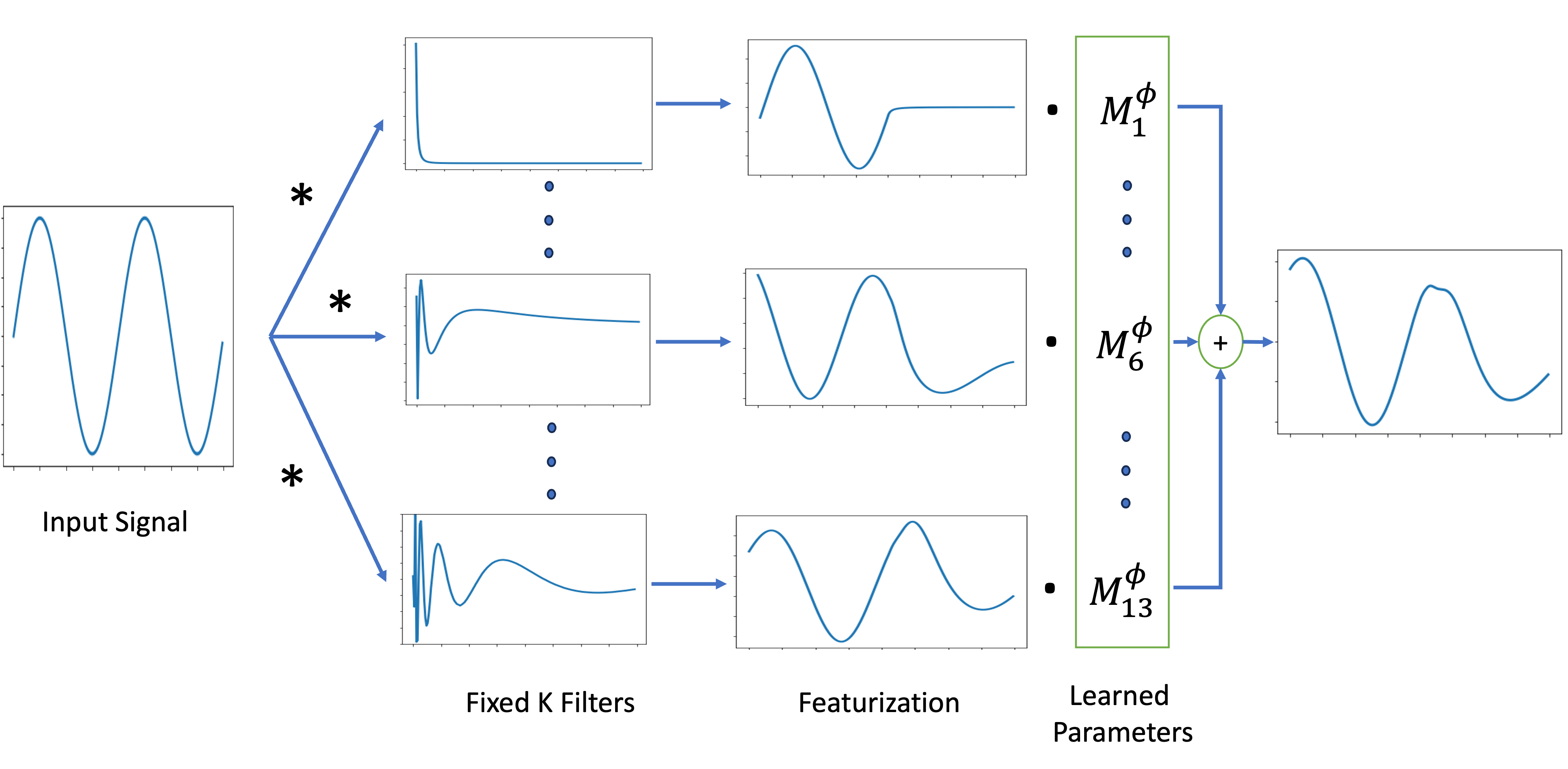
A schematic figure of the basic neural architecture called the Spectral Transform Unit (STU) is depictured in the following figure. More sophisticated variants including hybrid attention-STU architectures are also implemented and tested by the team.

Where do the filters come from?

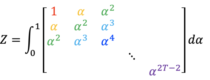
This section is a bit more mathematical, it gives only the gist of how the filters arise. The subspace that we would like to span is the set of all vectors that have the form $\mu_\alpha = [1 , \alpha, \alpha^2, … ]$, since these vectors naturally arise in the recursive application of a linear dynamical system. We thus consider a uniform distribution over these vectors, and the matrix $Z = \int_{\alpha = 0}^1 \mu_\alpha \mu_\alpha^\top$. This is a fixed matrix, unrelated to the data, that naturally arises from the structure of linear dynamics. It has a special property: it is a Hankle matrix, depicted below, and known theorems in mathematics show that its spectrum has an exponential decay property.

The filters we use are the eigenvectors correspnding to the largest eigenvalues of this matrix. For more details on how to extend this intuition to higher dimensions see this paper, extension to asymetric matrices, and detailed treatment in textbook.

Why is Spectral Filtering Important for Longer Memory?

The main advantage of spectral filtering applies to certain types of linear dynamical systems, in particular those with symmetric matrices, as follows. The effective memory (measured by the number of filters) required to represent an observation at any point in the sequence in the spectral basis is independent of the system memory parameter $\frac{1}{\delta}$!. This guarantee indicates that if we featurize the input into the spectral basis, we can potentially design models that are capable of efficiently and stably representing systems with extremely long memory even with effective memory approaching infinity $\frac{1}{\delta} \rightarrow \infty$. This striking fact motivates our derivation of the recurrent spectral architecture, and is the underlying justification for the performance and training stability gains we see in experiments.

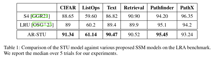
Experiments with neural architectures that make use of spectral filtering, which we call Spectral Transform Unit (STU), show promise on the long range arena benchmarks as follows:

For more details on the STU neural architecture, mathematical details on how the spectral filters are designed, as well as their theoretical properties, check out our recent paper!

Share on: