15 May 2023

Meta-optimization, adaptive gradient methods and parameter-free optimization

The study of mathematical optimization is a hallmark of the application of the scientific method to almost all engineering fields. With the rise of machine learning and large scale problems, attention shifted from interior point methods based on Newton’s method to first order methods (FOM). The most popular and efficient FOM are adaptive gradient methods (AGM), see chapter 6 of lecture notes here and explanations below.

Recent refinements to FOM, that are motivated by AGM, are adaptations that remove the need for fine-tuning of parameters. These include a flurry of recent papers, to give a short list:

and more that we have not covered here. The developments in mathematical programming that led to AGM and auto parameter tuning is rooted in the following fundamental question:

CAN WE AUTOMATICALLY FIND THE BEST OPTIMIZER FOR A GIVEN TASK?

In a recent work, we give a surprising positive answer to this question that stems from the same motivation as AGM, in a very general setting of mathematical optimization called meta-optimization. The solution proposed is based on a new formulation of optimization as online control, and makes crucial use of tools in a new methodology of online control called online nonstochastic control.

In this post we summarize this recent optimization framework and how it relates to AGM and parameter-free auto-tuning methods.

The motivation for meta-optimization

The motivation for meta-optimization is the question of how to learn the best optimizer for given tasks. We approach this question from an online convex optimization perspective:
In meta-optimization, the optimizer is given a sequence of N tasks, and can make T optimization steps per task. These tasks can be separate optimization problems, such as neural network training tasks, or online learning problems where data arrives iteratively in an online manner.

At each step, the optimizer suffers instantaneous costs, and the goal is to compete with the best optimization algorithm in hindsight in terms of total cost. We call the excess total cost the “meta-regret”, since this notion is analogous to the usual definition of regret in vanilla online optimization. If we can develop a method with sublinear meta-regret, then we can argue that this method converges to the cost of the best optimization algorithm on average, and compete with it.

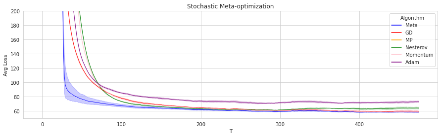
Here is an illustrative example: consider an optimization task of linear regression over random data, i.i.d. sampled from the same distribution. Such an interesting setting was proposed in this paper by Pedregosa and Scieur, where the motivation was to design the best FOM for a certain data distribution in linear regression problems. The plot below shows training error decrease as a function of time, where the error bars represent different trials. The band around meta-optimization shows that over time, the algorithm’s performance improves; meanwhile, there is almost no variation around the performance of the other methods. The meta-optimization approach improves over time as it learns the best optimizer for the task. Below we explain our approach in more detail.

Why is learning the learning rate hard?

Consider a restricted setting of learning the best optimizer, where we are given an optimization problem with T fixed learning rate gradient descent iterations, and the goal is to find the best learning rate to minimize the objective function at the last iteration. Finding the optimal gradient descent learning rate takes the form of the following minimization problem:

\[\min_\eta f(x_T),\ \ \text{subject to } x_{t+1} = x_t - \eta\nabla f(x_t).\]

We can unroll the minimization objective from the initial point $x_1$,

\[f(x_T) = f(x_1 - \eta\nabla f(x_1) - \eta\sum_{t=2}^{T-1} \nabla f(x_t)) = f(x_1 - \eta\nabla f(x_1) - \eta \nabla f(x_1 - \eta\nabla f(x_1)) - ...)\]

From this expression, it is clear that $f(x_T)$ is a nonconvex function of $\eta$. This means that the natural approach of applying FOM to the learning rate itself, for example hypergradient descent, is not guaranteed to converge to global optimality.

Meta-optimization methods guarantee competing with the global optimum for the learning rate from a set, for example in the case of convex quadratic objectives.

Online control for meta-optimization

The relationship between control and optimization spans decades: even the names of optimization algorithms, such as the “heavy ball method” and “momentum”, borrow from the realm of physical dynamical systems.

The analysis of mathematical optimization algorithms often makes use of control methodology. The most common application is that of the Lyapunov direct method for analyzing stability of a dynamical system. Lyapunov’s direct method involves creating an energy or potential function, also called the “Lyapunov function”. This function needs to be non-increasing along the trajectory of the dynamics, and strictly positive for states other than the equilibrium (global minimum for an optimization problem) to certify the stability of the system. A common example given in introductory courses on dynamics is that of the motion equations of the pendulum.

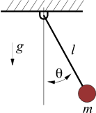
The Lyapunov function for this system is taken to be the total energy, kinetic and potential. Tedrake’s book provides an excellent exposition.

The connections between Lyapunov’s direct method for stability analysis and optimization were further explored by Lassard, Recht and Packard, and recently in the extensive thesis of Wilson. However, the direct method is less suited to our purpose of finding the best algorithm for a task. Most notably, the direct method is useful for analyzing existing methods, and does not come with a recipe for deriving/learning a task-specific algorithm.

An alternative to Lyapunov’s direct method is Lyapunov linearization, which approximates a dynamical system with a time-varying linear dynamical system. Linear dynamics are significantly better understood compared to nonlinear dynamical systems, especially after the work of Kalman on state space control and the Linear Quadratic Regulator. However, Lyapunov’s linearization is seldom used in the analysis of optimization methods, possibly due to the limitations of existing linear control methods. These methods typically assume the knowledge of system dynamics in advance, and efficient methods are only known for quadratic losses. Moreover, the noise in the system is commonly assumed to be stochastic, which is a restriction on the formulation of the dynamical system from optimization trajectories.

Here comes a new theory for online control that was recently developed in the machine learning literature: Online Nonstochastic Control (see also ICML tutorial and code therein). This new methodology can overcome these limitations of control for the design and analysis of optimization algorithms:

The framework is online and does not require a-priori knowledge of the dynamical system.
Efficient algorithms (such as GPC) exist for any convex costs.
The framework is regret-based, and allows for nonstochastic noise.

With the use of online nonstochastic control, we can model meta optimization as an iterative control problem and derive new efficient algorithms for learning the best algorithm for a sequence of optimization tasks! Not only that, techniques in online nonstochastic control provides a method to resolve the challenge of nonconvexity, which exists even for learning the learning rate as we explained before, through the use of convex relaxation.

Formalization of meta-optimization

The formal setting of meta-optimization is as follows. We are given a sequence of optimization problems, called episodes. The goal of the player is not only to minimize the total cost in each episode, but also to compete with a set of available optimization methods.

Specifically, in each of the N episodes, we have a sequence of T optimization steps that are either deterministic, stochastic, or online. At the beginning of an episode, the iterate is “reset” to a given starting point $x_{1, i}$. In the most general formulation of the problem, at time $(t, i)$, an optimization algorithm $A$ chooses a point $x_{t, i} \in K$, in a convex domain $K \subseteq R^d$. It then suffers a cost $f_{t, i}(x_{t, i})$. Let $x_{t, i}(A)$ denote the point chosen by $A$ at time $(t, i)$, and for a certain episode $i \in [N]$, denote the cost of an optimization algorithm $A$ by

\[J_i(A) = \sum_{t=1}^T f_{t, i}(x_{t, i}(A) ) - \min_{x^* \in K} \sum_{t=1}^T f_{t,i}(x^*) .\]

The standard goal in optimization, either deterministic, stochastic, or online, is to minimize each $J_i$ in isolation. In meta-optimization, the goal is to minimize the cumulative cost in both each episode, and overall in terms of the choice of the algorithm. We thus define the meta-regret to be

$\text{MetaRegret}(A) = \sum_{i=1}^N J_i(A) - \min_{A^* \in \Pi} \sum_{i=1}^N J_i(A^*) ,$ where $\Pi$ is the benchmark algorithm class. The meta-regret is the regret incurred for learning the best optimization algorithm in hindsight, and captures both efficient per-episode optimization as well as competing with the best algorithm in $\Pi$.

In a recent paper, we give efficient methods based on the GPC that guarantee meta-regret that scales as $O(\sqrt{NT})$ for meta optimization of quadratic functions. If the functions are convex smooth, the method has meta-regret scaling as $O((NT)^{¾})$ in expectation. In certain settings, this captures learning the learning rate for smooth optimization as a special case!

The search for the best algorithm for a given problem has a long history, and in the following sections, we take a look at the development of AGM and more recent parameter-free methods.

Adaptive gradient methods

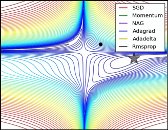
In the pursuit of learning the best optimizer, AGM is perhaps the biggest success story thus far. The theory of adaptive regularization is well-developed and highly active, and has led to numerous algorithmic refinements that have shaped the field of optimization for machine learning. Here is a nice illustration by Sebastian Ruder on adaptive optimizers vs. SGD, showing clear acceleration

http://ruder.io/optimizing-gradient-descent/

Adaptive optimizers reach state of the art in a variety of deep learning tasks, in both generalization and training error. But what is the theory behind them?

Let’s start from the textbook basics: stochastic gradient descent for non-smooth convex optimization. This is without loss of generality, since one can reduce the problem of finding an approximate local minimum of a smooth non-convex function (say the training error for a deep neural network) to iterated convex optimization (see Lemma A.21 here).

SGD has the following update rule

\[x_{t+1} \leftarrow x_t - \eta \tilde{\nabla}_t\]

Where $\tilde{\nabla}_t$ is a random estimator for the gradient (given by usually looking at only a few examples out of the training set). The textbook proof says that SGD for non-smooth convex optimization converges to the optimal solution at a rate of $O(\frac{ \sqrt{ \sigma^2 } }{\sqrt{T} } ).$

Here $\sigma^2$ is the variance of the stochastic gradient estimator, and T is the number of iterations. The variance has clear importance to the overall running time. This rate is optimal, and obtained by carefully tuning the learning rate $\eta$ to be inversely proportional to the variance, more precisely, $\eta = O(\frac{1}{\sqrt{t \sigma^2}})$. The proof of this fact is elementary, and details can be found in these lecture notes, chapter 2.

The intuition for adaptive regularization is now simple: consider an optimization problem, in which each coordinate is independent of the rest. It is reasonable to fine tune the learning rate for each coordinate separately - to achieve optimal convergence in that particular subspace of the problem, independently of the rest.

Thus, it is reasonable to change the SGD update rule to the more robust

\[x_{t+1} \leftarrow x_t - D_t \nabla_t ,\]

where $D_t$ is a diagonal matrix that contains in coordinate $(i,i)$ the learning rate for coordinate i in the gradient. Thus, the robust version of stochastic gradient descent should behave as the above equation, with the empirical variance on the diagonal of $D_t$,

\[D_t(i,i) = \frac{1}{\sqrt{\sum_{s < t} \nabla_s(i)^2}} .\]

This is exactly the diagonal version of the Adagrad algorithm!

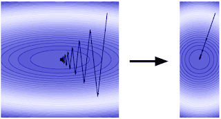
The intuition above can give rise to strong theorems about regularization in online learning. But what is regularization and why is it useful? Regularization can be seen as a method of transforming the geometry of the loss landscape in order to condition the optimization problem for faster first order optimization, as in the illustration below.

More formally, regularization changes the update rule of the algorithm at hand, and captures a variety of methods commonly known as Mirrored-Descent. The zoo of different regularizations raises an obvious question: which one is best? Reality, as always, is complicated: different data properties and different applications will render different algorithms better. This question directly relates to the motivating question for meta-optimization: which algorithm is best for the task, in a more limited setting.

The machine learning specialist has an equally obvious answer: can we learn the best regularization (or algorithm) on the fly? This is exactly the motivating question that gave rise to Adaptive Regularization! The Adagrad algorithm was the first to formalize this question, and prove that with a changing regularization, it can compete with the best algorithm in hindsight over the data (see chapter 5.6 here).

Parameter-free optimization: auto-tuning to the scale

Anyone with practical experience in optimization is aware of the need for hyperparameter tuning. Virtually all algorithms come with tunable parameters, and the practitioner needs to set these correctly to attain optimal behavior. Can we avoid this practice, and come up with completely automated methods?

This is a closely related question to the one we started with! Indeed, the relationship is more than superficial: the motivation for AGM is to automate the choice of the preconditioner. This solves part of the tuning problem, but the “scale” term remains, which is closely related to the distance of the initial point from the global optimum.

From a theoretical perspective, the goal is to obtain the optimal regret bound for online learning, which online gradient descent / Adagrad obtains depending on the geometry of the problem. However, not knowing the initial distance to optimality introduces logarithmic terms to the regret bound of Theorem 3.1 in this book. Removing this log term requires sophisticated machinery and different approaches have been applied, e.g.

coin-betting methods
using the empirical distance in lieu of diameter as per D-adaptation, DoG optimizer
Black-box reduction via online balancing as per Mechanic
Adaptive regret in SAMUEL

The motivation for these recent developments goes back to the original question we started with: CAN WE AUTOMATICALLY FIND THE BEST OPTIMIZER FOR A GIVEN TASK? The meta-optimization methodology addresses a significantly more general problem via different tools, and encompasses the learning of hyperparameters as well as preconditioners.

We hope this was a fun introduction to a new approach for learning the best algorithm, for more details, please see the full paper!

tags:
Share on: