New Methods in Control: The Gradient Perturbation Controller

The following post is based on this paper and this paper.

The mainstream thought in classical control operates under the simplifying principle that nature evolves according to well-specified dynamics perturbed by i.i.d. Gaussian noise, a field called Optimal Control. While this principle has proven very successful in some real world systems, it does not lend itself to the construction of truly robust controllers. In the real world one can expect all sorts of deviations from this setting, including:

• Inherent correlations between perturbations across time due to the environment.
• Modeling misspecification, which can introduce unforeseeable, non-stochastic deviations from the assumed dynamics.
• Completely adversarial perturbations introduced by a malicious entity.

Indeed, in the world of classical supervised learning, the presence of the above factors has led to the adoption of online learning in lieu of statistical learning, which allows for robust noise models and game-theoretic / strategic learning. A natural question arises: what is the analogue of online learning and worst-case regret in robust control?

Linear Dynamical Systems and Optimal Control

Dynamical systems constitute the formalism to describe time-dependent, dynamic real-world phenomenon, ranging from fluid flow through a pipe, the movement of a pendulum, to the change of weather. The archetypal example here is a linear dynamical system, which permits a particularly intuitive interpretation as a (configurable) vector field (from wikipedia):

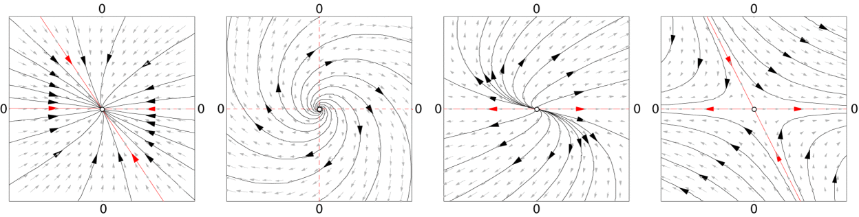
A linear dynamical system (LDS) posits the state of a system evolves via the following dynamical relation:

\[x_{t+1} = Ax_t + Bu_t + w_t\]

(video by @robertghrist)

Here \(x_t\) represents the state of the system, \(u_t\) represents a control input and \(w_t\) is a perturbation introduced to the dynamics, for the time step t. The vector fields above illustrate the behavior of the system for a few different choices of A, when the control input \(u_t\) is set to zero. The control inputs, when correctly chosen, can modify the dynamics to induce a particular desired behavior. For example, controlling the thermostat in a data center to achieve a particular temperature, applying a force to a pendulum to keep it upright, or driving a drone to a destination.

The goal of the controller is to produce a sequence of control actions \(u_1 \ldots u_T\) aimed at minimizing the cumulative loss \(\sum_t c_t(x_t, u_t)\). In classical control the loss functions are convex quadratics and known ahead of time. However, in the quest for more robust controllers, henceforth we will consider a broader class of general (possibly non-quadratic) convex cost functions, which may be adversarially chosen, and only be revealed online per-time-step to the controller.

Previous notions: LQR and H-infinity control

Perhaps the most fundamental setting in control theory is a LDS is with quadratic costs \(c_t\) and i.i.d Gaussian perturbations \(w_t\). The solution known as the Linear Quadratic Regulator, derived by solving the Riccati equation, is well understood and corresponds to a linear policy (i.e. the control input is a linear function of the state).

The assumption of i.i.d perturbations has been relaxed in classical control theory, with the introduction of a min-max notion, in a subfield known as \(H_{\infty}\) control. Informally, the idea behind \(H_{\infty}\) control is to design a controller which performs well against all sequences of bounded perturbations. There are two shortcomings of this approach; firstly computing such a controller can be a difficult optimization problem in itself. While a closed form for such a controller is known for linear dynamical systems with quadratic costs, no such form is known when costs can be non-quadratic. Secondly and perhaps more importantly, the min-max notion is non-adaptive and hence often too pessimistic. It is possible that during the execution of the system, nature produces a benign (predictable) sequence of perturbations (say, for instance, the perturbations are, in truth, highly correlated). The \(H_{\infty}\) controller in this setting could be overly pessimistic and lead to a higher cost than what could be achieved via a potentially more adaptive controller. This motivates our approach of minimizing regret, which we describe next.

A less pessimistic metric: Policy regret

Our starting point for more robust control is regret minimization in games. Regret minimization is a well-accepted metric in online learning, and we consider applying it to online control.

Formally, we measure the efficacy of a controller through the following notion of policy regret.

\[\mathrm{Regret} = \sum_{t} c_t(x_t, u_t) - \min_{\mathrm{stable } K} c_t(x_t(K), -Kx_t)\]

Here in, \(x_t(K)\) represents the state encountered when executing the linear policy \(K\). In particular, the second term represents the total cost paid by the best(in hindsight) stable linear policy had it executed in the system facing the same sequence of perturbations as the controller. In this regard the above notion of regret is counterfactual and hence more challenging than the more common stateless notion of regret.
(Remark: a stable linear policy K is one which ensures that the spectral radius of  A-BK is strictly less than one. For a formal quantitative definition, please see the paper.)

Furthermore, the choice of comparing to a linear policy is made keeping tractability in mind. Note that this nevertheless generalizes the standard Linear Quadratic Regulator and \(H_{\infty}\) control on Linear Dynamical Systems, as the optimal choice of controllers in those settings is indeed a linear policy (if the cost functions are quadratic, our setting allows more general loss functions).

Algorithms which achieve low regret on the above objective are naturally adaptive as they perform as well as the best controller (upto a negligible additive regret) oblivious to whether the sequence is friendly or adversarial.

A new type of controller

In successive recent works ([1] and [2]), we show that the above notion of policy regret is tractable and can be sublinear (even logarithmic under certain conditions). Using a new parameterization for controller that we detail next, we obtain the following results:

• Robustness to Adversarial Perturbations ([1]) – For arbitrary, but bounded, perturbations \(w_t\), which may even be chosen adversarially, we provide an efficient algorithm that achieves regret of \(O(\sqrt{T})\).
• Fast Rates under Stochastic Perturbations ([2]) – Further, for strongly convex costs, and i.i.d. perturbations, we give an efficient algorithm with a poly-logarithmic (in T) regret guarantee.

The former result is the first such result to establish vanishing average regret in an online setting for control with adversarial perturbations. The latter result offers a significant improvement over the work of Cohen et al. who established a rate of \(O(\sqrt{T})\) in a similar (stochastic) setting.

We assume that the dynamical system i.e. (A,B) is completely known to us and the state is fully observable. These assumptions have been eliminated in further work with our collaborators, and will be a subject of a future blog post. We now describe the core ideas which go into achieving both our results.

The Gradient Perturbation Controller

Consider how the choice of the linear controller determines the control input.

The above display demonstrates that the action, state, and hence the cost are non-convex functions of the linear controller K. The first piece of our result evades this lack of convexity by over-parametrization, ie. relaxing the notion of a linear policy as described next.

In place of learning a direct representation of a linear controller K, we learn a sequence of matrices \(M_1, M_2 \ldots\) which represent the dependence of \(u_t\) on \(w_{t - i}\) under the execution of some linear policy. Schematically, we parameterize our policy as follows

Note that, the assumption that the dynamics is known permits the exact inference of \(w_t\)’s and thereby making the execution of such a controller possible. While the choice of the controller ensures that control inputs are linear in \(\{M_i\}\), the superposition principle for linear dynamical systems ensures that the state sequence too is linear in the same variables. Therefore, the cost of execution of such a controller parameterized via \(\{M_i\}\) is convex and we can hope to learn them using standard techniques like Gradient Descent. Observe that, by construction, it is possible to emulate the behavior any linear controller K by a suitable choice of \(\{M_i\}\)’s.

There are two barriers though. First, the number of parameters grows with time \(T\) and so can regret and running time. Secondly, since there is a state, the decision a controller makes at a particular instance affects the future. We deal with these two problems formally in the paper and show how they may be circumvented. One of the important techniques we use is Online Convex Optimization with Memory.

With all the core components in place, we provide a brief specification of our algorithm. Let’s fix some memory length H, and a time step t. Define a proxy cost as

\(c_t(M_1, \ldots M_H) = \textrm{Cost Paid at Time }t\textrm{, had we execute the policy }\{M_1, \ldots M_H\}\) for \(t-H\) steps, with the system reset to \(0\).

The algorithm now as suggested by Anava, Hazan and Manor, is to take a gradient step on the above proxy.

The above algorithm achieves \(O(\sqrt{T})\) regret against worst-case noise. For the full proof and the precise derivation of the algorithm, check out the paper.

Achieving Logarithmic Regret

Algorithms for (state-less) online learning often enjoy logarithmic regret guarantees in the presence of strongly convex loss functions. Prima facie, one could hope that for dynamical systems with strongly convex costs, such a stronger regret guarantee would hold. The cautionary note here is that strong convexity of the cost \(c_t(x_t, u_t)\) in the control input does not imply strong convexity in the controller representation.,

In fact, the strong convexity of our proxy cost function \(c(M_1, \ldots M_H)\) in its natural parameterization over M’s is further hindered by the fact that the space of M’s constitutes a highly over-parametrized representation (say, vs. K). Indeed in the case of adversarial perturbations, it is easy to construct a case where the strong convexity does not transfer over from the control to the controller.

In a future blog post we detail how this technical difficulty can be overcome using the natural gradient method, giving rise to a logarithmic regret algorithm for control.

Experimental Validation

Below we provide empirical evaluations of the GPC controller in various scenarios, demonstrating it is indeed more robust to correlated noise than previous notions. (All the plots below are produced by a new research-first control and time series library in the works — Alpha version scheduled to be released soon! STAY TUNED!!!)

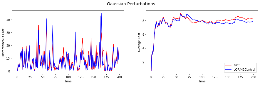
To start, let’s reproduce the classical setting of controlling an LDS with i.i.d. Gaussian noise. Here, the LQR program is optimal. Yet, the plot below attests that our new control methodology offers a slightly suboptimal, yet comparable, performance. This observation also underlines the message the the proposed controller tracks the optimal controller without any foreknowledge of the structure of the perturbations. Here, for example, GPC is not made aware of the i.i.d. nature of the perturbations.

Moving on to correlated perturbations across time, a simple such setting is when the perturbations are drawn from a Gaussian Random Walk (as opposed to independent Gaussians). Note that here it is possible to derive the optimal controller via the separation principle. Here is the performance plot:

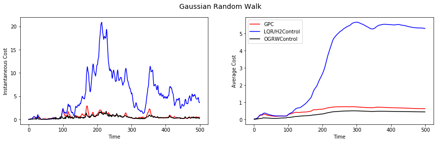
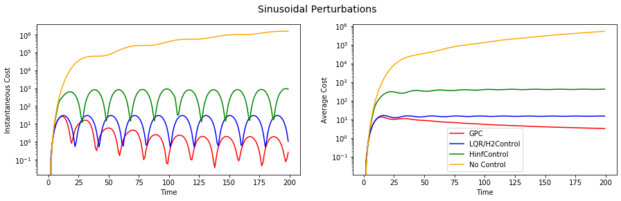
Note that the default LQR controller performs much worse, where as GPC is able to track the performance of the optimal controller quite closely. Next up, sinusoidal noise:

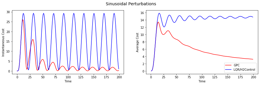
Here the full power of regret minimization is exhibited as the consecutive samples of the sine function are very correlated, yet predictable. GPC vastly outperforms LQR as one would expect. But, is this fundamentally a hard setting? What would happen if we use the H-infinity controller, or, god forbid, no control at all? We see this in the next plot (on the log-linear scale):

What’s next?

We have surveyed a new family of controls that are fundamentally different than classical optimal control: they are adaptive and attain regret guarantees vs. adversarial noise. Their preliminary experimental tests seem quite promising.

In the coming posts we will:

1. Explain how GPC can obtain the first logarithmic regret in the tracking/Kalman setting,
2. Reveal our new research-first library for control / time-series prediction,
3. Tackle more general settings.

Stay tuned! Preferably using the GPC… 🙂

Share on: