Boosting for Dynamical Systems

In a famous 1906 competition at a local fair in Plymouth, England, participants were asked to guess the weight of an ox. Out of a crowd of hundreds, no one came close to the ox’s actual weight, but the average of all guesses was almost correct. How is it that combining the opinions of laymen can somehow arrive at highly reasoned decisions, despite the weak judgment of individual members? This concept of harnessing wisdom from weak rules of thumb to form a highly accurate prediction rule, is the basis of ensemble methods and boosting. Boosting is a theoretically sound methodology that has transformed machine learning across a variety of applications; in classification and regression tasks, online learning, and many more.

In the case of online learning, examples for training a predictor are not available in advance, but are revealed one at a time. Online boosting combines a set of online prediction rules, or weak learners. At every time step, each weak learner outputs a prediction, suffers some loss and is then updated accordingly. The performance of an online learner is measured using the regret criterion, which compares the accumulated loss over time with that of the best fixed decision in hindsight. A Boosting algorithm can choose which examples are fed to each of the weak learners, as well as the losses they incur. Intuitively, the online booster can encourage some weak learners to become really good in predicting certain common cases, while allowing others to focus on edge cases that are harder to predict. Overall, the online boosting framework can achieve low regret guarantees based on the learners’ individual regret values.

However, online learning can become more challenging when our actions have consequences on the environment. This can be illustrated with the following experiment: imagine learning to balance a long pole on your hand. When you move your hand slightly, the pole tilts. You then move your hand in the opposite direction, and it bounces back and tilts to the other side. One jerk the wrong way might have you struggling for a good few seconds to rebalance. In other words, a sequence of decisions you made earlier determines whether or not the pole is balanced at any given time, rather than the single decision you make at that point.

More generally, consider cases when our environment has a state, and is in some sense “remembering” our past choices. A stateful framework, able to model a wide range of such phenomena, is a dynamical system. A dynamical system can be thought of as a function that determines, given the current state, what the state of the system will be in the next time step. Think of the physical dynamics that determines our pole’s position based on sequential hand movements. Other intuitive examples are the fluctuations of stock prices in the stock market, or the local weather temperatures; these can all be modeled with dynamical systems.

So how can boosting help us make better predictions for a dynamical system? In recent work we propose an algorithm, which we refer to as DynaBoost, that achieves this goal. In the paper we provide theoretical regret bounds, as well as an empirical evaluation in a variety of applications, such as online control and time-series prediction.

Learning for Online Control

Control theory is a field of applied mathematics that deals with the control of various physical processes and engineering systems. The objective is to design an action rule, or controller, for a dynamical system such that steady state values are achieved quickly, and the system maintains stability.

Consider a simple Linear Dynamical System (LDS):

\[x_{t+1} = A x_t + B u_t + w_t\]

where \(x_t,u_t\) are the state and control values at time t, respectively. Assume a known transition dynamics specified by the matrices A and B, and an arbitrary disturbance to the system given by \(w_t\). The goal of the controller is to minimize a convex cost function \(c_t(x_t,u_t)\).

A provably optimal controller for the Gaussian noise case (where \(w_t\) are normally distributed) and when the cost functions are quadratic, is the Linear Quadratic Regulator (LQR). LQR computes a pre-fixed matrix K such that \(u_t^{LQR} = K x_t\). In other words, LQR computes a linear controller – which linearly maps the state into a control at every time step.

A recent advancement in online control considers arbitrary disturbances, as opposed to normally distributed noise. In this more general setting, there is no closed form for the optimal controller. Instead, it is proposed to use a weighted sum of previously observed noises, i.e., \(u_t^{WL} = K x_t + \sum_{i=1}^H M_i w_{t-i}\) , where \(M_1,...,M_H\) are learned parameters, updated in an online fashion. This method is shown to attain vanishing average regret compared to the best fixed linear controller in hindsight, and is applicable for general convex cost functions as opposed to only quadratics.

Crucially, the state-dependent term \(Kx_t\) is not learned. Since the learned parameters of the above controller therefore considers only a fixed number of recent disturbances, we can apply existing online convex optimization techniques developed for learning with loss functions that have bounded memory.

Boosting for Online Control

Using the insights described above to remove state in online control, we can now use techniques from online boosting. DynaBoost maintains multiple copies of the base-controller above, with each copy corresponding to one stage in boosting. At every time step, the control \(u_t\) is obtained from a convex combination of the base-controllers’ outputs \(u_t^{WL(1)},...,u_t^{WL(N)}\). To update each base-controller’s parameters, DynaBoost feeds each controller with a residual proxy cost function, and seeks to obtain a minimizing point in the direction of the residual loss function’s gradient. Stability ensures that minimizing regret over the proxy costs (which have finite memory) suffices to minimize overall regret. See our paper for the detailed description of the algorithm and its regret guarantees.

Sanity check experiment

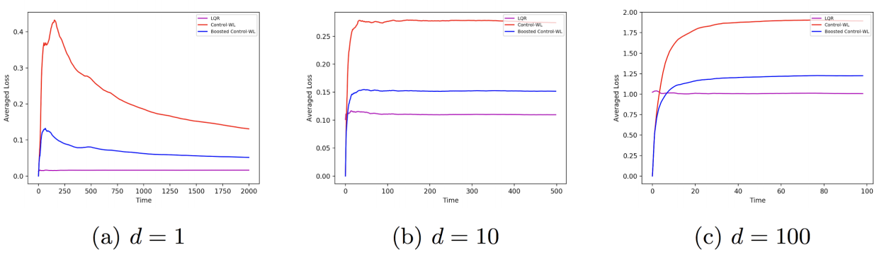
We first conducted experiments for the standard LQR setting with i.i.d. Gaussian noise and known dynamics. We applied our boosting method to the non-optimal controller with learned parameters (Control-WL), and we observe that boosting improves its loss and achieves near-optimal performance (here the optimal controller is given by the fixed LQR solution). We have tested an LDS of different dimensions \(d = 1,10,100\), and averaged results over multiple runs.

Correlated noise experiment

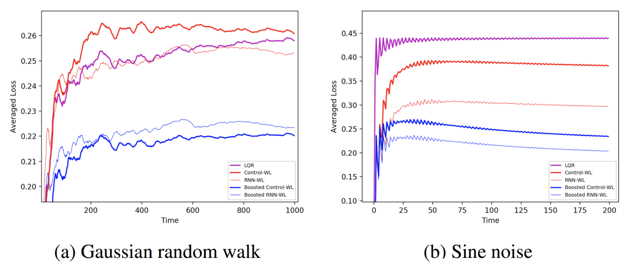
When the disturbances are not independently drawn, the LQR controller is not guaranteed to perform optimally. We experimented with two LDS settings with correlated disturbances in which (a) the disturbances \(w_t\) are generated from a Gaussian random-walk, and (b) where they are generated by a sine function applied to the time index. In these cases, boosted controllers perform better compared to the “weak” learned controller, and can also outperform the fixed LQR solution. We have also tested a Recurrent Neural Network, and observed that boosting is effective for RNNs as well.

Inverted Pendulum experiment

A more challenging experiment with a non-linear dynamical system is the Inverted Pendulum experiment. This is very similar to the pole balancing example we discussed above, and is a standard benchmark for control methods. The goal is to balance the inverted pendulum by applying torque that will stabilize it in a vertically upright position, in the presence of noise. In our experiments, we used correlated disturbances from a Gaussian random-walk. We follow the dynamics implemented in OpenAI Gym, and test the performance of different controllers: LQR, a learned controller, and boosting. The video below visualizes this experiment:

When averaging the loss value over multiple experiment runs, we get the following plot:

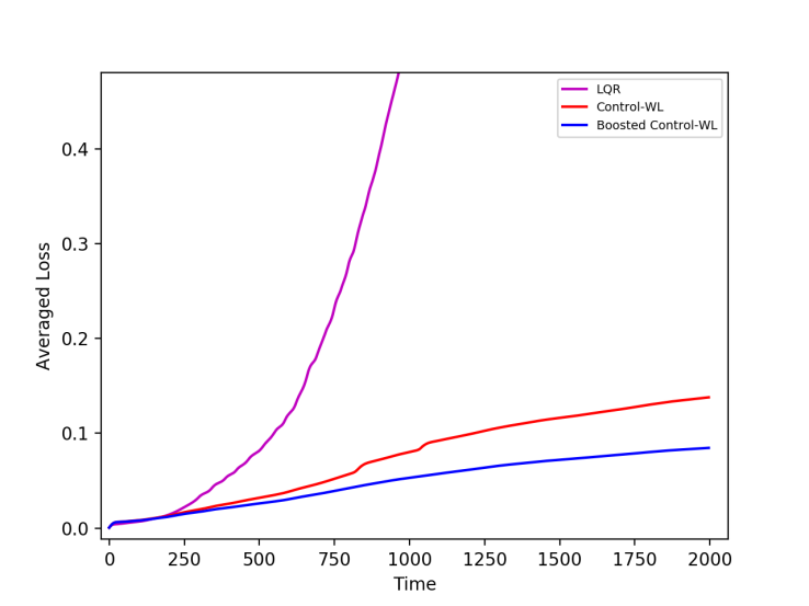
It can be seen that the learned controller performs much better than the LQR in the presence of correlated noise, and that boosting can improve its stability and achieve lower average loss.

Boosting for Time-Series Prediction

Similarly to the control setting, in time-series prediction tasks it is sufficient to use fixed horizons, and online boosting can be efficiently applied here as well. In time-series prediction, the data is often assumed to be generated from an autoregressive moving average (ARMA) model:

\[x_{t} = \sum_{i=1}^k \alpha_i x_{t-i} + \sum_{j=1}^q \beta_j w_j + w_t\]

In words, each data point \(x_t\) is given by a weighted sum of previous points, previous noises and a new noise term \(w_t\), where \(\alpha,\beta\) are the coefficients vectors.

To test our boosting method, We experimented with 4 simulated settings: 1) normally distributed noises, 2) coefficients of the dynamical system slowly change over time, 3) a single, abrupt, change of the coefficients, and, 4) correlated noise: Gaussian random walk.

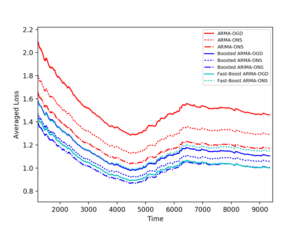
The weak learners tested here are the ARMA-ONS (online newton step) and ARMA-OGD (online gradient descent) algorithms for time-series prediction (See this paper for more details). We applied our boosting method, as well as a fast version of it, which applies to quadratic loss functions (we used squared difference in this case).

1) Gaussian Noise 2) Changing Coefficients

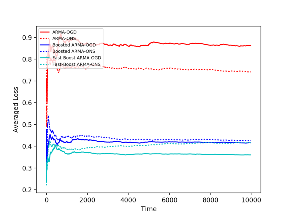
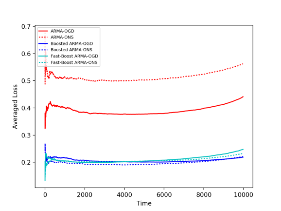
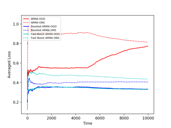
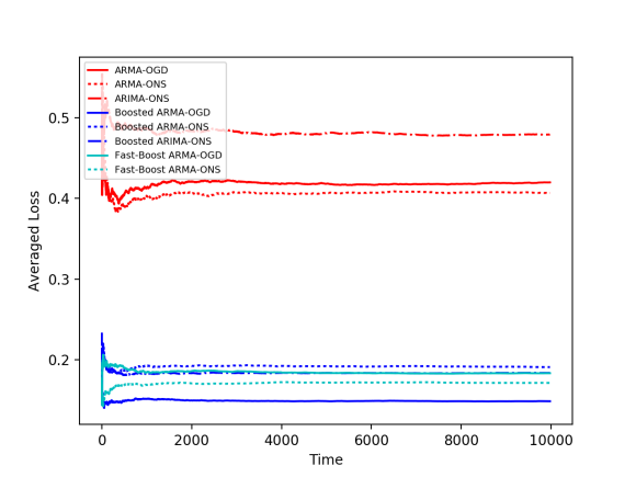
3) Abrupt Change 4) Correlated Noise

We can see in the plots above that all weak learners’ loss values (red) can be improved by online boosting methods (blue). A similar observation arises when experimenting with real-world data; we experimented with the Air Quality dataset from the UCI Machine Learning repository, that contains hourly averaged measurements of air quality properties from an Italian city throughout one year, as measured by chemical sensors. We apply similar weak learners to this task, as well as our boosting algorithms. Here we again obtain better averaged losses for boosted methods (blue) compared to the baselines (red).

Share on: