The complexity zoo and reductions in optimization

The following dilemma is encountered by many of my friends when teaching basic optimization: which variant/proof of gradient descent should one start with? Of course, one needs to decide on which depth of convex analysis one should dive into, and decide on issues such as “should I define strong-convexity?”, “discuss smoothness?”, “Nesterov acceleration?”, etc.

This is especially acute for courses that do not deal directly with optimization, which is described as a tool for learning or as a basic building block for other algorithms. Some approaches:

• I teach online gradient descent, in the context of online convex optimization, and then derive the offline counterpart. This is non-standard, but permits an extremely simple derivation and gets to the online learning component first.
• Sanjeev Arora teaches basic offline GD for the smooth and strongly-convex case first.
• In OR/optimization courses the smooth (but not strongly-convex) case is many times taught first.

All of these variants have different proofs whose connections are perhaps not immediate. If one wishes to go into more depth, usually in convex optimization courses one covers the full spectrum of different smoothness/strong-convexity/acceleration/stochasticity regimes, each with a separate analysis (a total of 16 possible configurations!)

This year I’ve tried something different in COS511 @ Princeton, which turns out also to have research significance. We’ve covered basic GD for well-conditioned functions, i.e. smooth and strongly-convex functions, and then extended these result by reduction to all other cases! A (simplified) outline of this teaching strategy is given in chapter 2 of this book.

Classical Strong-Convexity and Smoothness Reductions

Given any optimization algorithm A for the well-conditioned case (i.e., strongly convex and smooth case), we can derive an algorithm for smooth but not strongly functions as follows.

Given a non-strongly convex but smooth objective \(f\), define a objective by \(\text{strong-convexity reduction:} \qquad f_1(x) = f(x) +  \epsilon \|x\|^2\) It is straightforward to see that \(f_1\) differs from \(f\) by at most \(\epsilon\) times a distance factor, and in addition it is \(\epsilon\)-strongly convex. Thus, one can apply \(A\) to minimize \(f_1\) and get a solution which is not too far from the optimal solution for \(f\) itself.  This simplistic reduction yields an almost optimal rate, up to logarithmic factors.

Similar simplistic assumptions can be derived for (finite-sum forms of) non-smooth by strongly-convex functions (via randomized smoothing or Fenchel duality), and for functions that are neither smooth nor strongly-convex by just applying both reductions simultaneously. Notice that such classes of functions include famous machine learning problems such as SVM, Logistic Regression, SVM, L1-SVM, Lasso, and many others.

Necessity of Reductions

This is not only a pedagogical question. In fact, very few algorithms apply to the entire spectrum of strong-convexity / smoothness regimes, and thus reductions are very often intrinsically necessary. To name a few examples,

• Variance-reduction methods such as SAG, SAGA and SVRG require the objective to be smooth, and do not work for non-smooth problems like SVM. This is because for loss functions such as hinge loss, no unbiased gradient estimator can achieve a variance that approaches to zero
• Dual methods such as SDCA or APCG require the objective to be strongly convex, and do not directly apply to non-strongly convex problems. This is because for non-strongly convex objectives such as Lasso, their duals are not even be well-defined.
• Primal-dual methods such as SPDC require the objective to be both smooth and SC.

Optimality and Practicality of Reductions

The folklore strong-convexity and smoothing reductions are suboptimal. Focusing on the strong-convexity reduction for instance:

• It incurs a logarithmic factor log(1/ε) in the running time so leading to slower algorithms than direct methods. For instance, if \(f(x)\) is smooth but non-strongly convex, gradient descent minimizes it to an \(\epsilon\) accuracy in \(O(1/\epsilon)\) iterations; if one uses the reduction instead, the complexity becomes \(O(\log(1/\epsilon)/\epsilon)\).
• More importantly, algorithms based on such reductions become biased: the original objective value \(f(x)\) does not converge to the global minimum, and if the desired accuracy is changed, one has to change the weight of the regularizer \(\|x\|^2\) and restart the algorithm.

These theoretical concerns also translate into running time losses and parameter tuning difficulties in practice. For such reasons, researchers usually make efforts on designing unbiased methods instead.

• For instance, SVRG in theory solves the Lasso problem (with smoothness L) in time \(O((nd+\frac{Ld}{\epsilon})\log\frac{1}{\epsilon})\) using reduction. Later, direct and unbiased methods for Lasso are introduced, including SAGA which has running time \(O(\frac{nd+Ld}{\epsilon})\), and SVRG++ which has running time \(O(nd \log\frac{1}{\epsilon} + \frac{Ld}{\epsilon})\).

One can find academic papers derive various optimization improvements many times for only one of the settings, leaving the other settings desirable. An optimal and unbiased black-box reduction is thus a tool to extend optimization algorithms from one domain to the rest.

Optimal, Unbiased, and Practical Reductions

In this paper, we give optimal and unbiased reductions. For instance, the new reduction, when applied to SVRG, implies the same running time as SVRG++ up to constants, and is unbiased so converges to the global minimum. Perhaps more surprisingly, these new results imply new theoretical results that were not previously known by direct methods. To name two of such results:

• On Lasso, it gives an accelerated running time \(O(nd \log\frac{1}{\epsilon} + \frac{\sqrt{nL}d}{\sqrt{\epsilon}})\) where the best known result was not only an biased algorithm but also slower \(O( (nd + \frac{\sqrt{nL}d}{\sqrt{\epsilon}}) \log\frac{1}{\epsilon} )\).
• On SVM with strong convexity \(\sigma\), it gives an accelerated running time \(O(nd \log\frac{1}{\epsilon} + \frac{\sqrt{n}d}{\sqrt{\sigma \epsilon}})\) where the best known result was not only an biased algorithm but also slower \(O( (nd + \frac{\sqrt{n}d}{\sqrt{\sigma \epsilon}}) \log\frac{1}{\epsilon} )\).

These reductions are surprisingly simple. In the language of strong-convexity reduction, the new algorithm starts with a regularizer \(\lambda \|x\|^2\) of some large weight \(\lambda\), and then keeps halving it throughout the convergence. Here, the time to decrease \(\lambda\) can be either decided by theory or by practice (such as by computing duality gap).

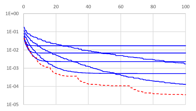
A figure to demonstrate the practical performance of our new reduction (red dotted curve) as compared to the classical biased reduction (blue curves, with different regularizer weights) are presented in the figure below.

As a final word – if you were every debating whether to post your paper on ArXiV, yet another example of how quickly it helps research propagate:  only a few weeks after our paper was made available online, Woodworth and Srebro have already made use of our reductions in their new paper.

Share on: