Making second order methods practical for machine learning

First-order methods such as Gradient Descent, AdaGrad, SVRG, etc. dominate the landscape of optimization for machine learning due to their extremely low per-iteration computational cost. Second order methods have largely been ignored in this context due to their prohibitively large time complexity. As a general rule, any super-linear time operation is prohibitively expensive for large scale data analysis. In our recent paper we attempt to bridge this divide by exhibiting an efficient linear time second order algorithm for typical (convex) optimization problems arising in machine learning.

Previously, second order methods were successfully implemented in linear time for special optimization problems such as maximum flow [see e.g. this paper] using very different techniques. In the optimization community, Quasi-Newton methods (such as BFGS) have been developed which use first order information to approximate a second order step. Efficient implementations of these methods (such as L-BFGS) have been proposed, mostly without theoretical guarantees.

Concretely, consider the PAC learning model where given \(m\) samples \(\{(\mathbf{x}_k, y_k)\}_{k\in \{1,\dots, m\}}\) the objective is to produce a hypothesis from a hypothesis class that minimizes the overall error. This optimization problem, known as  Empirical Risk Minimization, can be written as follows: \(\min_{\theta \in \mathbb{R}^d} f(\theta) = \min_{\theta \in \mathbb{R}^d} \left\{\frac{1}{m}\sum\limits_{k=1}^m f_k(\theta) + R(\theta) \right\}.\) In typical examples of interest, such as Logistic Regression, soft-margin Support Vector Machines, etc., we have that each \(f_k(\theta)\) is a convex function of the form \(\ell(y_k, \theta^{\top}\mathbf{x}_k)\) and \(R(\theta)\) is a regularization function. For simplicity, consider the Euclidean regularization given by \(R(\theta) = \lambda \|\theta\|^2\).

Gradient Descent is a natural first approach to optimize a function, whereby you repeatedly take steps in the direction opposite of the gradient at the current iterate \(\mathbf{x}_{t+1} = \mathbf{x}_t -- \eta \nabla f(\mathbf{x}_t).\) Under certain conditions on the function and with an appropriate choice of \(\eta\), it can be shown this process converges linearly to the true minimizer \(\mathbf{x}^*\). If \(f\) has condition number \(\kappa\), then it can be shown that \(O(\kappa \log (1/\epsilon))\) iterations are needed to be \(\epsilon\)-close to the minimizer, with each iteration taking \(O(md)\) time, so the total running time is \(O(md \kappa \log(1/ \epsilon))\). Numerous extensions to this basic method have been proposed in the ML literature in recent years, which is a subject for a future blog post.

Given the success of first order methods, a natural extension is to incorporate second order information in deciding what direction to take at each iteration. Newton’s Method does exactly this, where, denoting \(\nabla^{-2}f(\mathbf{x}) := [\nabla^2 f(\mathbf{x})]^{-1}\), the update takes the form \(\mathbf{x}_{t+1} = \mathbf{x}_t -- \eta \nabla^{-2}f(\mathbf{x}_t) \nabla f(\mathbf{x}_t).\) Although Newton’s Method can converge to the optimum of a quadratic function in a single iteration and can achieve quadratic convergence for general functions (when close enough to the optimum), the per-iteration costs can be prohibitively expensive. Each step requires calculation of the Hessian (which is \(O(md^2)\) for functions of the form \(f(\mathbf{x})  = \sum\limits_{k=1}^m f_k(\mathbf{x})\)) as well as a matrix inversion, which naively takes \(O(d^3)\) time.

Drawing inspiration from the success of using stochastic gradient estimates, a natural step forward is to use stochastic second order information in order to estimate the Newton’s direction. One of the key hurdles towards a direct application of this approach is the lack of an immediate unbiased estimator of the inverse Hessian. Indeed, it is not the case that the inverse of an unbiased estimator of the Hessian is an unbiased estimator of the Hessian inverse. In a recent paper by Erdogdu and Montanari, they propose an algorithm called NewSamp, which first obtains an estimate of the Hessian by aggregating multiple samples, and then computes the matrix inverse. Unfortunately the above method still suffers due to the prohibitive run-time of the matrix inverse operation. One can take a spectral approximation to speed up inversion, however this comes at the cost of loosing some spectral information and thus loosing some nice theoretical guarantees.

Our method tackles these issues by making use of the Neumann series. Suppose that, for all \(\mathbf{x}\), \(\|\nabla^2 f(\mathbf{x})\|_2 \leq 1\),  \(\nabla^2 f(\mathbf{x}) \succeq 0\). Then, considering the Neumann series of the Hessian matrix, we have that \(\nabla^{-2}f(\mathbf{x}) = \sum\limits_{i=0}^{\infty} \left(I -- \nabla^2 f(\mathbf{x})\right)^i.\) The above representation can be used to construct an unbiased estimator in the following way. The key component is an unbiased estimator of a single term \(\left(I -- \nabla^2 f(\mathbf{x})\right)^i\) in the above summation. This can obtained by taking independent and unbiased samples \(\{ \nabla^2 f_{[j]} \}\) and creating the product by multiplying the individual terms. Formally, pick a probability distribution \(\{p_i\}_{i \geq 0}\) over the non-negative integers (representing a probability distribution over the individual terms in the series) and sample an index \(\hat{i}\). Sample \(\hat{i}\) independent and unbiased Hessian samples \(\left\{\nabla^2 f_{[j]}(\mathbf{x})\right\}_{j \in \{1, \dots, \hat{i}\}}\) and define the estimator: \(\tilde{\nabla}^{-2} f(\mathbf{x}) = \frac{1}{p_{\hat{i}}} \prod\limits_{j=1}^{\hat{i}} \left(I -- \nabla^2 f_{[j]}(\mathbf{x})\right).\) Note that the above estimator is an unbiased estimator which follows from the fact that the samples are independent and unbiased.

We consider the above estimator in our paper and analyze its convergence. The above estimator unfortunately has the disadvantage that it captures one term in the summation and introduces the need for picking a distribution over the terms. However, this issue can be circumvented by making the following observation about a recursive reformulation of the above series:

\(\nabla^{-2} f = I + \left(I -- \nabla^2 f\right)\left( I + \left(I -- \nabla^2 f\right) ( \ldots)\right).  \) If we curtail the Taylor series to contain the first \(t\) terms (which is equivalent to the recursive depth of \(t\) in the above formulation) we can see that an unbiased estimator of the curtailed series can easily be constructed given \(t\) unbiased and independent samples as follows:

\(\nabla^{-2} f = I + \left(I -- \nabla^2 f_{[t]}\right)\left( I + \left(I -- \nabla^2 f_{[t-1]}\right) ( \ldots)\right).\) Note that as \(t \rightarrow \infty\) our estimator becomes an unbiased estimator of the inverse. We use the above estimator in place of the true inverse in the Newton Step in the new algorithm, dubbed LiSSA.

The next key observation we make with regards to our estimator is that since we are interested in computing the Newton direction \((\nabla^{-2} f \nabla f)\), we need to repeatedly compute products of the form \((I -- \nabla^2 f_{[i]})v\) where \(\nabla^2 f_{[i]}\) is a sample of the Hessian and \(v\) is a vector. As remarked earlier in common machine learning settings the loss function is usually of the form \(\ell_k(y_k, \theta^{\top} \mathbf{x}_k)\) and therefore the hessian is usually of the form \(c \mathbf{x}_k\mathbf{x}_k^{\top}\), i.e. it is a rank 1 matrix. It can now be seen that the product \((I -- \nabla^2 f_{[i]})v\) can be performed in time \(O(d)\), giving us a linear time update step. For full details, we refer the reader to Algorithm 1 in the paper.

We would like to point out an alternative interpretation of our estimator. Consider the second order approximation \(g(\mathbf{y})\) to the function \(f(\mathbf{x})\) at any point \(\mathbf{z}\), where \(\mathbf{y} = \mathbf{x} -- \mathbf{z}\), given by \(g(\mathbf{y}) = f(\mathbf{z}) + \nabla f(\mathbf{z})^{\top}\mathbf{y} + \frac{1}{2}\mathbf{y}^{\top}\nabla^2 f(\mathbf{z})\mathbf{y}.\) Indeed, a single step of Newton’s method takes us to the minimizer of the quadratic. Let’s consider what a gradient descent step for the above quadratic looks like: \(\mathbf{x}_{t+1} = (I -- \nabla^2 f(\mathbf{z}))\mathbf{x}_t -- \nabla f(\mathbf{z}).\) It can now be seen that using \(t\) terms of the recursive Taylor series as the inverse of the Hessian corresponds exactly to doing \(t\) gradient descent steps on the quadratic approximation. Continuing the analogy we get that our stochastic estimator is a specific form of SGD on the above quadratic. Instead of SGD, one can use any of the improved/accelerated/variance-reduced versions too. Although the above connection is precise we note that it is important that in the expression above, the gradient of \(f\) is exact (and not stochastic). Indeed, known lower bounds on stochastic optimization imply that it is impossible to achieve the kind of guarantees we achieve with purely stochastic first and second order information. This is the reason one cannot adapt the standard SGD analysis in our scenario, and it remains an intuitive explanation only.

Before presenting the theorem governing the convergence of LiSSA, we will introduce some useful notation. It is convenient to first assume WLOG that every function \(f_k(\mathbf{x})\) has been scaled such that \(\|\nabla^2 f_k(\mathbf{x})\| \leq 1.\) We also denote the condition number of \(f(\mathbf{x})\) as \(\kappa\), and we define \(\kappa_{max}\) to be such that \(\lambda_{min}(\nabla^2 f_k(\mathbf{x})) \geq \frac{1}{\kappa_{max}}.\)

Theorem:  LiSSA returns a point \(\mathbf{x}_t\) such that with probability at least \(1 -- \delta\), \(f(\mathbf{x}_t) \leq \min\limits_{\mathbf{x}^*} f(\mathbf{x}^*) + \epsilon\) in \(O(\log \frac{1}{\epsilon})\) iterations, and total time \(O \left( \left( md + \kappa_{max}^2 \kappa d \right) \log \frac{1}{\epsilon}\right).\)

At this point we would like to comment on the running times described above. Our theoretical guarantees are similar to methods such as SVRG and SDCA which achieve running time \(O(m + \kappa)d\log(1/\epsilon)\). The additional loss of \(\kappa^2_{max}\) in our case is due to the concentration step as we prove high probability bounds on our per-step guarantee. In practice we observe that this concentration step is not required, i.e. applying our estimator only once, performs well as is demonstrated by the graphs below. It is remarkable that the number of iterations is independent of any condition number – this is the significant advantage of second order methods.

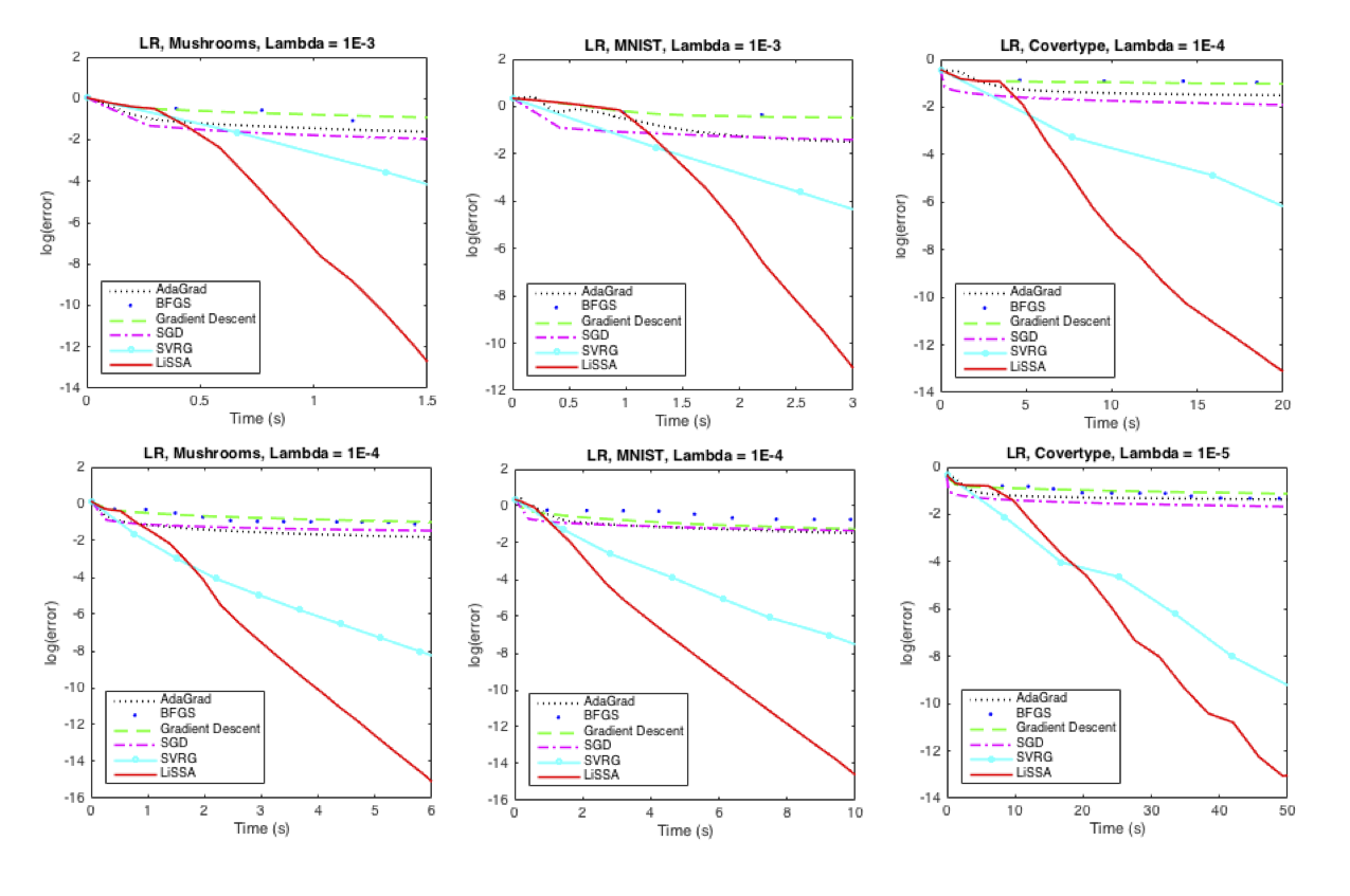
These preliminary experimental graphs compare LiSSA with standard algorithms such as AdaGrad, Gradient Descent, BFGS and SVRG on a binary Logistic Regression task on three datasets obtained from LibSVM. The metric used in the above graphs is log(Value – Optimum) vs Time Elapsed.

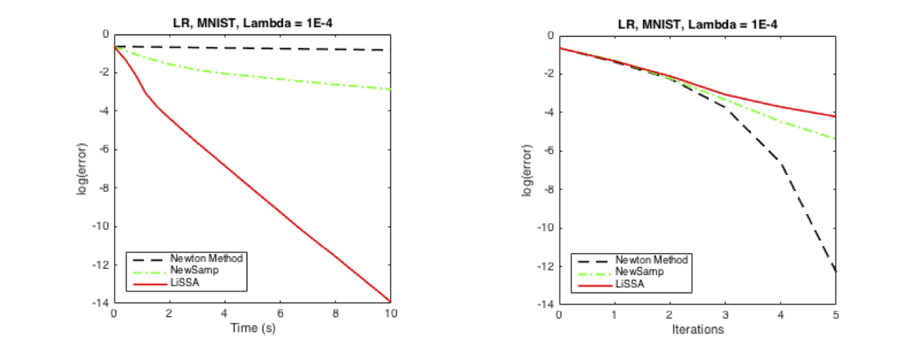
Next we include a comparison between LiSSA and second order methods, vanilla Newton’s Method and NewSamp. We observe that in terms of iterations Newton’s method shows a quadratic decline whereas NewSamp and LiSSA perform similarly in a linear fashion. As is expected, a significant performance advantage for LiSSA is observed when we consider a comparison with respect to time.

To summarize, in this blog post we described a linear time stochastic second order algorithm that achieves linear convergence for typical problems in machine learning while still maintaining run-times theoretically comparable to state-of-the-art first order algorithms. This relies heavily on the special structure of the optimization problem that allows our unbiased hessian estimator to be implemented efficiently, using only vector-vector products.

Share on: